ΔT is the difference between Terrestrial Time, TT, and Universal Time, UT1. TT provides a uniform time scale for astronomical calculations; UT1 follows Earth’s rotation. Earth’s rotation varies, so the difference has to be measured for recent dates and estimated for future ones.
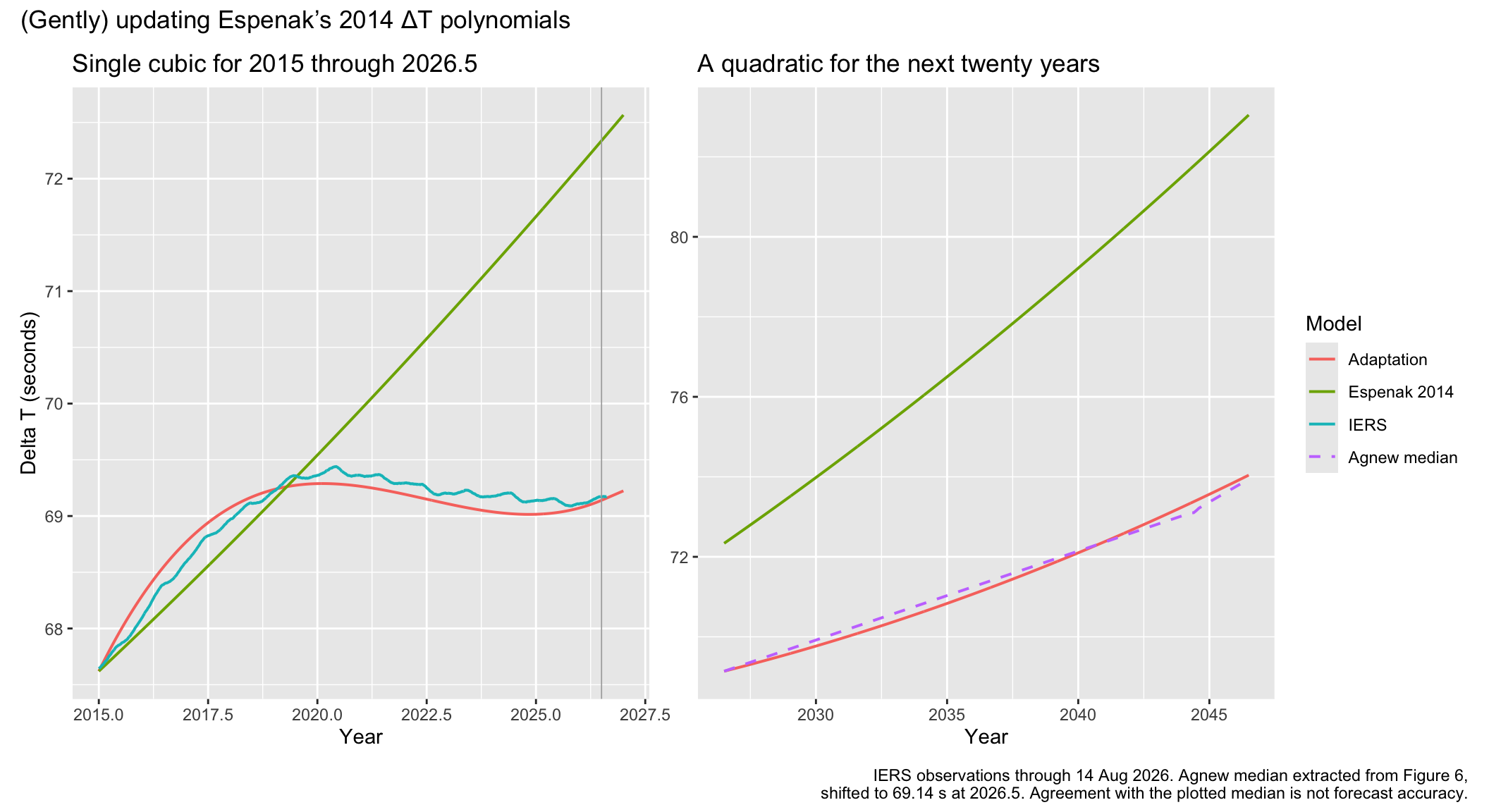
The 2014 ΔT polynomials published by the late Fred Espenak, based on earlier work with Jean Meeus, provide an easy way to get ΔT values aligned with historical observations and predictions. However, they need an update for recent and future dates. The 2014 expression gives about 72.3 seconds for mid-2026, compared with an observed value around 69.1 seconds. ΔT has grown much less than the formula predicted.
I want to see whether a small modification could improve this while keeping the expressions simple. The aim is to cover the past decade and use recent research to choose a reasonable extrapolation for the next ten or twenty years. I’m neither a geophysicist nor an astronomer; this is a practical adjustment for use in software. A few tenths of a second of fitting error would be acceptable.
Fitting the replacement polynomials
For the observations, I used the IERS C04 daily series, downloaded on 14 September 2026, with data through 14 August. These give UT1−UTC, which can be converted to ΔT using the known TAI−UTC offset and the fixed 32.184-second difference between TT and TAI. (Leap seconds in 2015 and 2016 need to be accounted for when doing this over the whole interval.)
There has been useful work since 2014. Malkin’s 2024 paper provides a polynomial with periodic terms that can be checked against subsequent observations. Using its published coefficients without refitting, I get an RMS error of about 0.055 seconds over the two years following its fitting interval. That is quite good. For June 2026, though, its prediction is already some 0.1 seconds above the observed ΔT. It seems risky to simply extrapolate this particular result for another twenty years.
For that longer interval, Agnew’s 2026 paper, The future(s) of UT1: a geophysical discussion, looks more useful. It combines models of the different contributions to Earth’s rotation and produces 8,000 simulations of its possible future behaviour. Figure 6 in the paper shows the median and the spread of the results through 2100.
I used that median as a reference for the next twenty years. This makes the choice depend on one published model by one author, with its assumptions. It would be difficult to claim a scientific consensus for a particular set of polynomial coefficients, especially for a layman like myself.
I extracted the median curve from Figure 6 and shifted it to start at ΔT = 69.14 seconds in mid-2026.
The resulting future expression is nicely unremarkable. For decimal year , let :
The quadratic coefficient, 0.0039755, is unchanged from Espenak’s expression. Keeping it avoids estimating long-term curvature from a short stretch of a graph. With that coefficient fixed, I fitted the linear coefficient by least squares to the shifted median, sampled every 0.1 year over 2026.5–2046.5. This gives about 0.1656 seconds per year. This is a compromise over the whole twenty-year interval; it should not be read as a measurement of the current rate of change.
The expression stays within about 0.3 seconds of the shifted, plotted median over that interval. That is close enough for this purpose.
The recent past needs a separate expression. A single cubic covers 2015 to mid-2026 reasonably well. With :
I also fitted the cubic by least squares, using the daily IERS observations with equal weight. Fixing its values at both ends and its final slope to match the future branch leaves just to fit; the constraints determine and . Its RMS error is 0.12 seconds, and its largest absolute error is 0.21 seconds. It rises a bit too quickly at first and dips a bit too far later on. Adding more pieces improves the fit, but the extra complication doesn’t seem worthwhile.
The branches before 2015 stay as they are in Fred Espenak’s EclipseWise version. The cubic joins their value at 2015, though its slope is different. At 2026.5, the cubic and quadratic match in both value and slope.
The replacement branches, with in seconds and the decimal year, are:
where and . The fitted slopes are approximately
With years, the length of the cubic’s interval, the remaining coefficients follow from the endpoint values and final slope:
The calculations use full-precision coefficients. With the rounded and shown here, calculate and from the formulas above to preserve the matching value and slope at the join.
Some example values, in seconds:
| Year | Adaptation | Espenak 2014 |
|---|---|---|
| 2030 | 69.8 | 74.0 |
| 2035 | 70.8 | 76.5 |
| 2040 | 72.1 | 79.2 |
| 2045 | 73.6 | 82.1 |
| 2050 | 75.2 | 85.2 |
| 2100 | 102.8 | 127.3 |
Comparisons and uncertainty
The US Naval Observatory also publishes “long-term” ΔT predictions. Its table, downloaded on 14 September 2026, ends at 2033.75 and does not state when the forecast was issued. The product page says “from finals.data”, but I could not find a description of how the long-term extrapolation is calculated. Comparing the values directly, without any further fitting:
| Year | USNO | Adaptation | Espenak 2014 |
|---|---|---|---|
| 2027.00 | 69.14 | 69.22 | 72.57 |
| 2030.00 | 69.97 | 69.77 | 73.98 |
| 2033.00 | 70.98 | 70.38 | 75.47 |
| 2033.75 | 71.25 | 70.55 | 75.85 |
USNO predicts somewhat faster growth in the early 2030s. At the end of its table, it is about 0.7 seconds above the adaptation. Both are well below Espenak’s original expression. This is a useful comparison of forecasts; we will have to wait to see how either fares against observations.
The cubic’s errors are measured against observations; the future expression’s differences are measured against Agnew’s plotted median. Following that curve closely does not establish accuracy in 2040.
Agnew’s spread of possible outcomes makes this fairly clear:
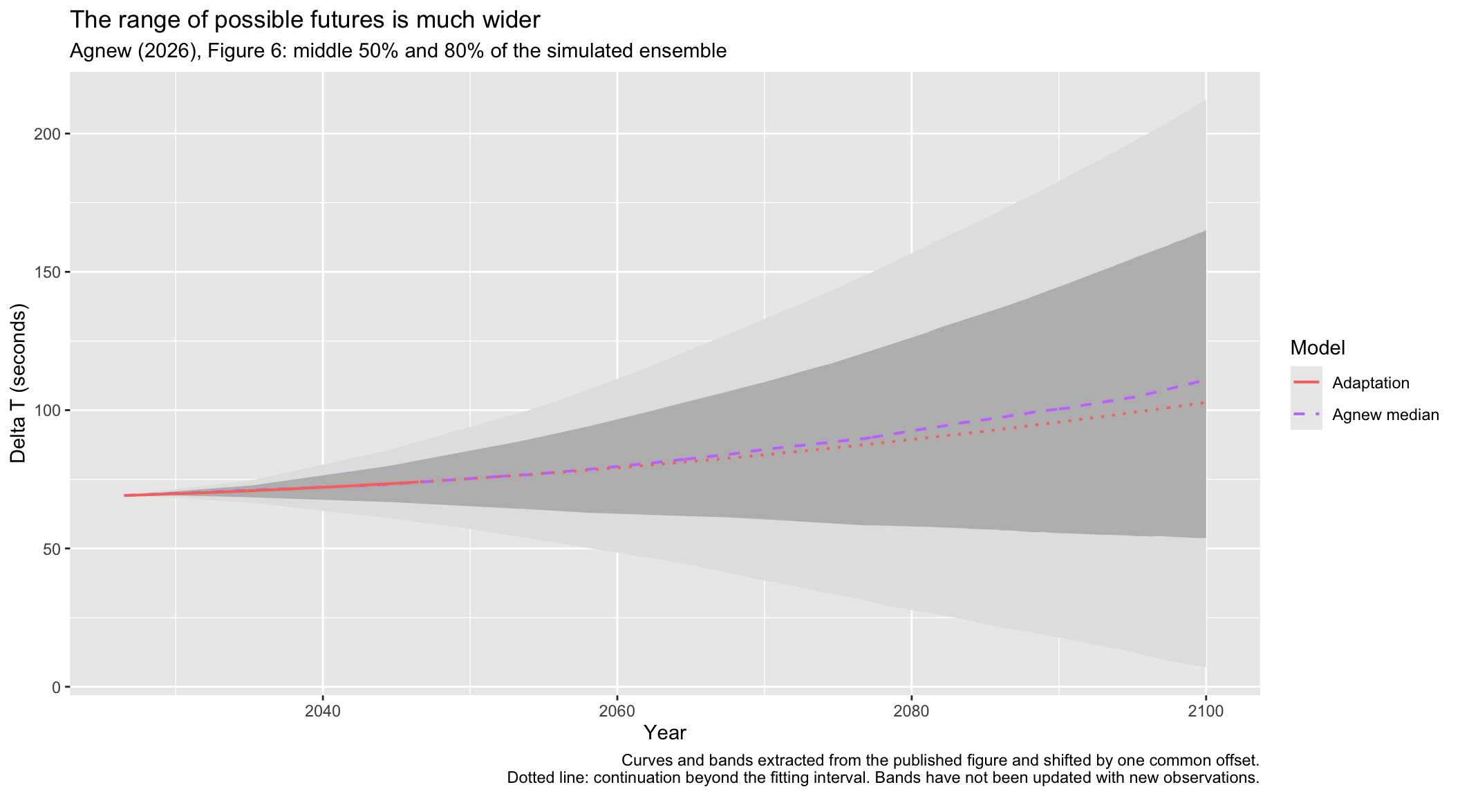
By 2045, the shifted middle 80% of the simulations spans roughly 60.5 to 86.4 seconds. I applied the same constant shift to all the plotted bounds; I have not rerun the simulations with newer observations. These bands describe Agnew’s model and its assumptions.
The formula will return a value all the way to the year 3000. That is useful for software, but I have no evidence that this modification improves on Espenak’s values for the distant future. The fit covers twenty years; retaining his quadratic coefficient does not make it a reliable prediction for the next thousand. A value for 2100 or 3000 could be substantially wrong.
For recent dates and the next decade or two, this still seems a more useful default than continuing to use the old future branch unchanged.