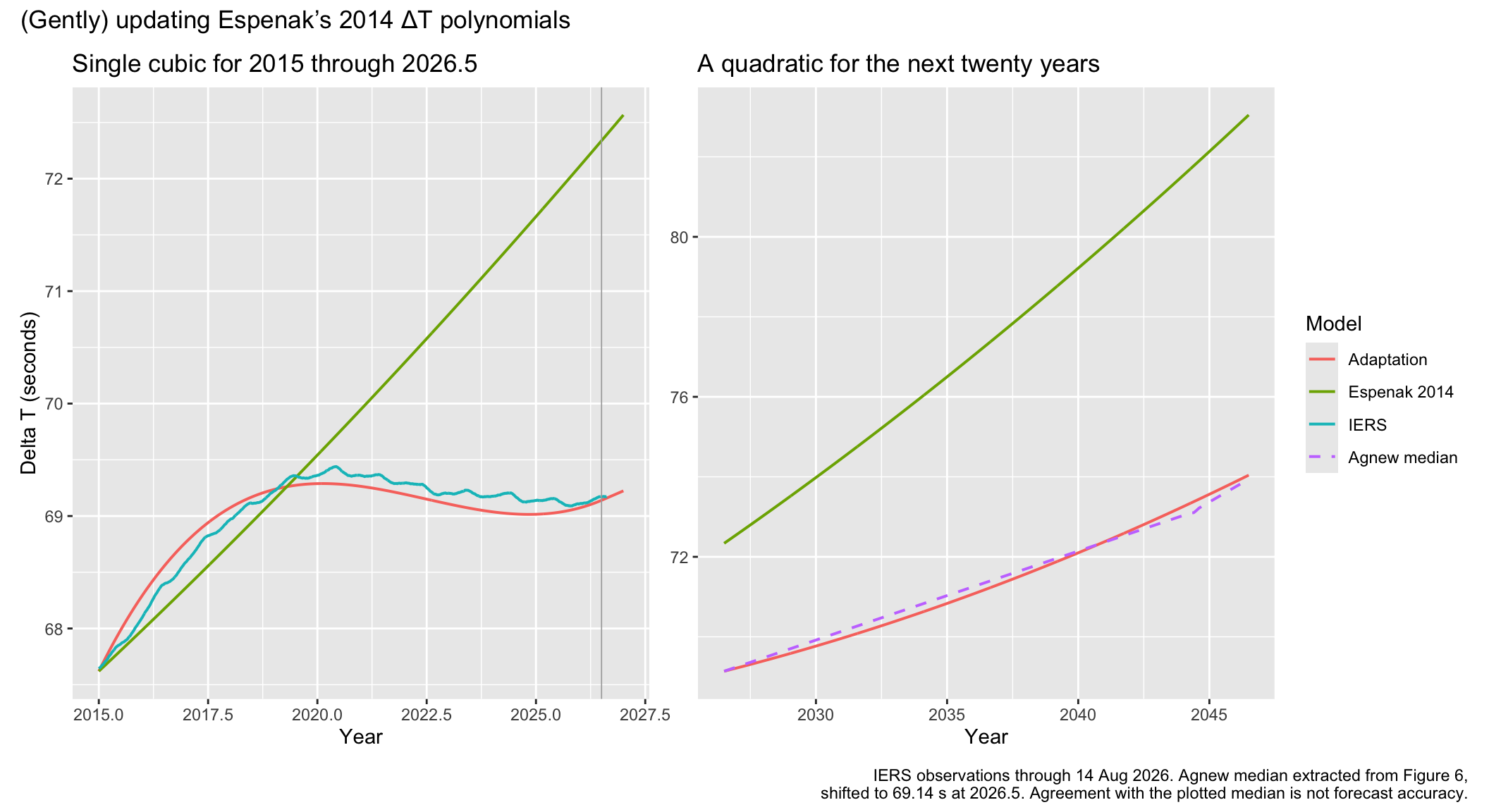
(Gently) updating Espenak’s ΔT polynomials – Klaus Brunner’s personal website

The 2014 ΔT polynomials published by the late Fred Espenak, based on earlier work with Jean Meeus, could use a modest update. For mid-2026, they give about 72.3 seconds, compared with an observed value around 69.2 seconds. I’d like to improve the estimates for recent and future dates while keeping the expressions simple.

The idea is to cover the past decade and use recent research to guide the extrapolation over the next twenty years or so. I’m neither a geophysicist nor an astronomer; this is a practical adjustment for use in software.

What is ΔT?

ΔT is the difference between Terrestrial Time (TT), a uniform time scale for astronomical calculations, and Universal Time (UT1), which follows Earth’s rotation. Unfortunately, Earth’s rotation varies in ways that are not fully understood and difficult to predict. The polynomials provide a simple estimate of ΔT for a given date.

Fitting the replacement polynomials

For the observations, I used the IERS C04 daily series, downloaded on 14 September 2026, with data through 14 August. These give UT1−UTC, which can be converted to ΔT using the known TAI−UTC offset and the fixed 32.184-second difference between TT and TAI. (The TAI−UTC offset changes whenever a leap second is added.)

For historical ΔT, Morrison and colleagues’ 2021 update provides an alternative based on cubic splines, with published coefficients extending through 2019.

But what about the future? For short-term prediction, Malkin’s 2024 paper provides a polynomial with periodic terms. Using its published coefficients without refitting, I get a root mean square (RMS) error of about 0.055 seconds over the two years following its fitting interval. That is quite good. By June 2026, its prediction is about 0.1 seconds above the observed ΔT. The paper examines a two-year forecast; extrapolating for another twenty seems risky.

For longer-term extrapolation, Agnew’s 2026 paper, The future(s) of UT1: a geophysical discussion, looks more useful. It combines models of the different contributions to Earth’s rotation and produces 8,000 simulations of its possible future behaviour. Figure 6 in the paper shows the median and the spread of the results through 2100.

Duncan Agnew kindly supplied an updated numerical series (personal communication, 19 September 2026), using IERS data through July.

I used its median as a reference through 2100. Fitting to it gives a systematic way to choose the coefficients, though the result depends on this one model and its assumptions. It would be difficult to claim a scientific consensus for a particular set of polynomial coefficients, especially for an amateur like myself.

I fixed the join between the historical and future expressions at ΔT = 69.14 seconds in mid-2026, close to the observed value. The future expression is nicely unremarkable. For decimal year $y$ , let $t=y-2026.5$ :

$\Delta T = 69.14 + st + qt^2.$

I fitted $s$ and $q$ by least squares to the supplied median at 0.1-year intervals from 2026.6 to 2100. The expression stays within about 0.14 seconds of the supplied median over the first twenty years, and 0.52 seconds through 2100. Close enough for this purpose.

The recent past needs a separate expression. A single quartic covers 2015 to mid-2026 reasonably well. With $x=y-2015$ :

$\Delta T = 67.62 + ax + bx^2 + cx^3 + dx^4.$

I also fitted the quartic by least squares, using the daily IERS observations with equal weight. Matching the values and slopes of the neighbouring branches at both ends fixes $a=0.2930$ and leaves only $d$ to fit; the constraints determine $b$ and $c$ . Its RMS error is 0.11 seconds, and its largest absolute error is 0.22 seconds. Letting the slope at 2015 vary would give a closer fit overall, but I’m happy to trade a little accuracy for a smooth join.

Figure 1: Fit to the observations and Agnew’s median.

The branches before 2015 stay as they are in Espenak’s EclipseWise version. The expressions match in both value and slope at 2015 and 2026.5.

The replacement branches, with $\Delta T$ in seconds and $y$ the decimal year, are:

$\Delta T(y) = \begin{cases} 67.62 + ax + bx^2 + cx^3 + dx^4, & 2015 \le y < 2026.5, \\ 69.14 + st + qt^2, & 2026.5 \le y \le 3000, \end{cases}$

where $x = y - 2015$ and $t = y - 2026.5$ . The coefficients are

$\begin{aligned} a &= 0.2930, \qquad d \approx 0.0009758, \\ s &\approx 0.2880529, \qquad q \approx 0.0057380. \end{aligned}$

With $h=2026.5-2015=11.5$ years, the length of the quartic’s interval, the remaining coefficients follow from the endpoint values and final slope:

$\begin{aligned} b &= \frac{3(69.14-67.62)/h - 2a - s}{h} + dh^2 \approx 0.0875317, \\ c &= \frac{2(67.62-69.14)/h + a + s}{h^2} - 2dh \approx -0.0200498. \end{aligned}$

Full-precision coefficients for all intervals are in the appendix. Some example values, in seconds:

Year	Adaptation	Espenak 2014
2030	70.2	74.0
2035	72.0	76.5
2040	74.1	79.2
2045	76.4	82.1
2050	79.1	85.2
2100	121.3	127.3

Comparisons and uncertainty

The US Naval Observatory publishes “long-term” ΔT predictions. The table, downloaded on 14 September 2026, ends at 2033.75 and does not state when the forecast was issued. The product page says “from finals.data”, but I was unable to find a description of how the long-term extrapolation is calculated. Comparing the values directly, without any further fitting:

Table 1: Comparison with USNO predictions, in seconds.

Year	USNO	Adaptation	Espenak 2014
2027.00	69.14	69.29	72.57
2030.00	69.97	70.22	73.98
2033.00	70.98	71.25	75.47
2033.75	71.25	71.53	75.85

USNO predicts less growth than the adaptation. Its final entry is about 0.3 seconds below the adaptation. Both are well below Espenak’s original expression.

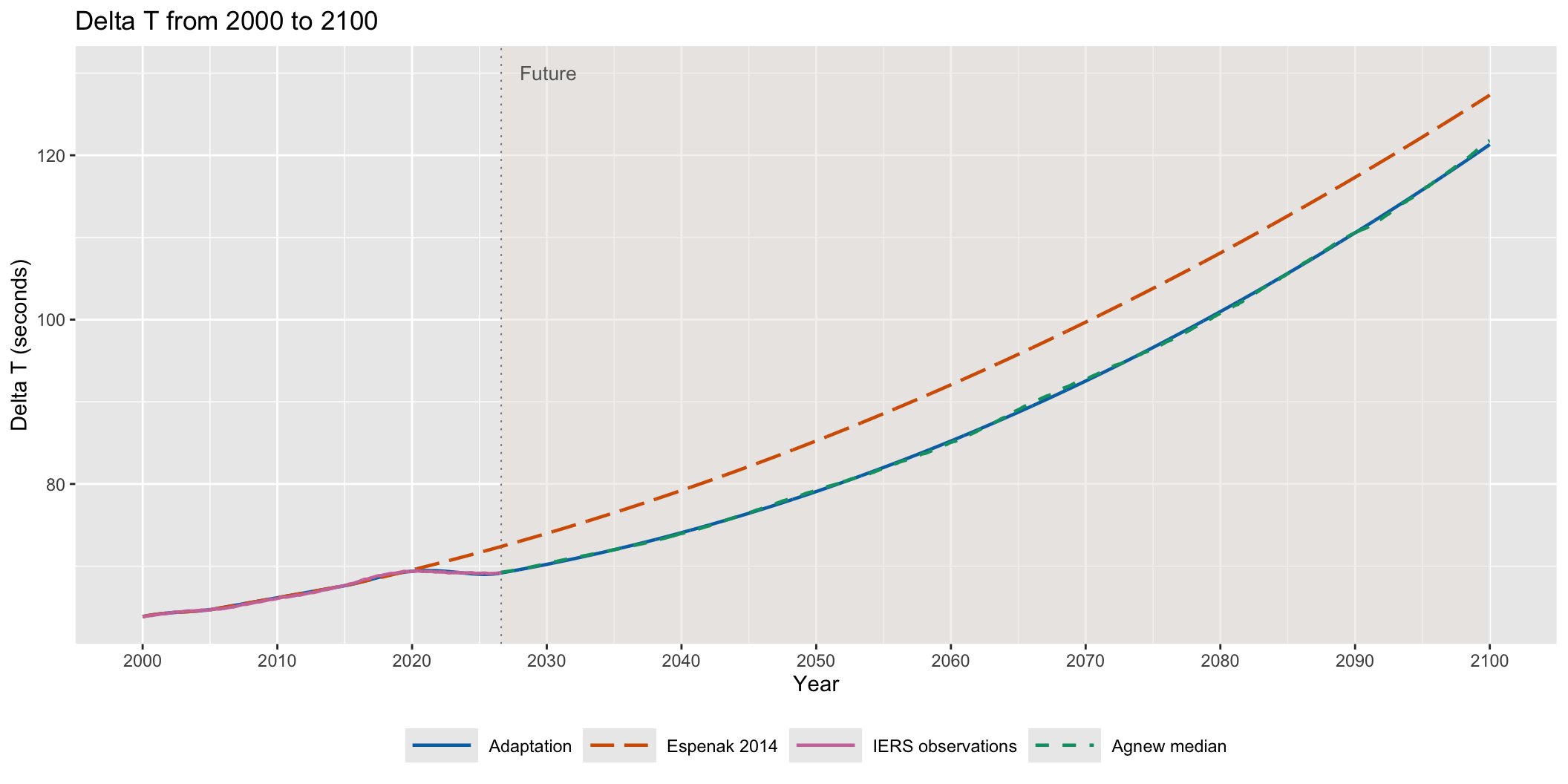
The quartic’s errors are measured against observations; the future expression’s differences are measured against Agnew’s simulated median.

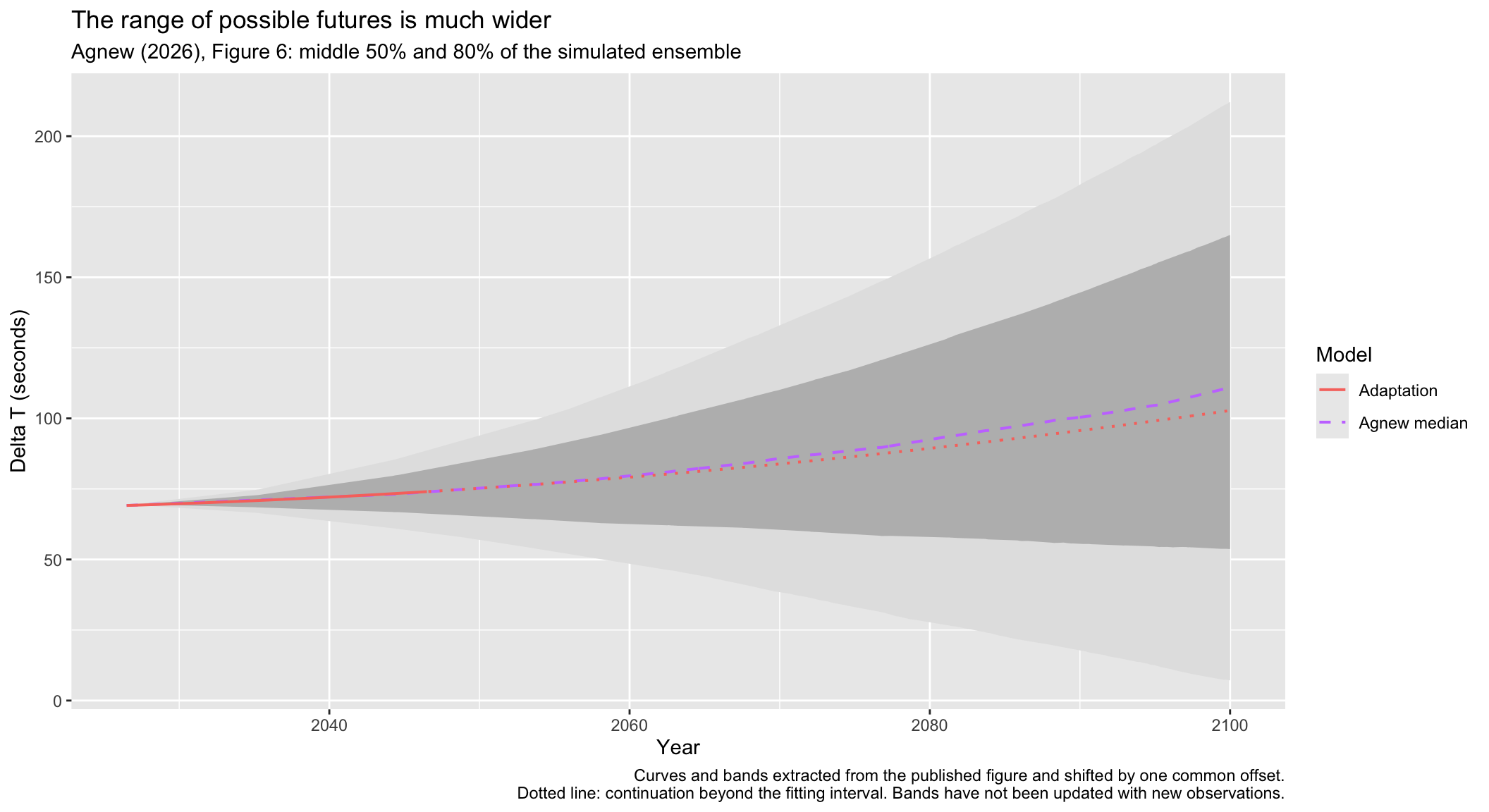
Figure 3: Agnew’s updated simulation ranges.

For 2045, the middle 80% of Agnew’s updated simulations lie between roughly 64.5 and 88.7 seconds. That spread is much wider than the fitting error and reflects the assumptions in his model.

As in the original Espenak/Meeus polynomials, the formula will return a value all the way to the year 3000. That is useful for software, but I have no idea if this modification improves on Espenak’s values for the distant future. Fitting a simulated median through 2100 does not make it a reliable prediction for the next thousand years. I would take it as an educated guess, at best.

For recent dates and the next couple of decades though, this adaptation seems a more useful default than continuing to use the old future branch unchanged.

Many thanks to Duncan Agnew for his help and for sharing the updated simulation results!

Appendix: Complete polynomials

The complete coefficient table includes Espenak’s historical branches. For decimal year $y$ , use the listed $t$ and coefficients in

$\Delta T = c_0 + c_1t + c_2t^2 + \cdots + c_7t^7.$

ΔT is in seconds; coefficients not listed are zero. Year 0 means 1 BCE.

Complete coefficient table

Interval	$t$	Coefficients
$-1999 \le y < -500$	$(y-1820)/100$	$c_0=-20$ , $c_2=32$
$-500 \le y < 500$	$y/100$	$c_0=10583.6$ , $c_1=-1014.41$ , $c_2=33.78311$ , $c_3=-5.952053$ , $c_4=-0.1798452$ , $c_5=0.022174192$ , $c_6=0.0090316521$
$500 \le y < 1600$	$(y-1000)/100$	$c_0=1574.2$ , $c_1=-556.01$ , $c_2=71.23472$ , $c_3=0.319781$ , $c_4=-0.8503463$ , $c_5=-0.005050998$ , $c_6=0.0083572073$
$1600 \le y < 1700$	$y-1600$	$c_0=120$ , $c_1=-0.9808$ , $c_2=-0.01532$ , $c_3=1/7129$
$1700 \le y < 1800$	$y-1700$	$c_0=8.83$ , $c_1=0.1603$ , $c_2=-0.0059285$ , $c_3=0.00013336$ , $c_4=-1/1174000$
$1800 \le y < 1860$	$y-1800$	$c_0=13.72$ , $c_1=-0.332447$ , $c_2=0.0068612$ , $c_3=0.0041116$ , $c_4=-0.00037436$ , $c_5=0.0000121272$ , $c_6=-0.0000001699$ , $c_7=0.000000000875$
$1860 \le y < 1900$	$y-1860$	$c_0=7.62$ , $c_1=0.5737$ , $c_2=-0.251754$ , $c_3=0.01680668$ , $c_4=-0.0004473624$ , $c_5=1/233174$
$1900 \le y < 1920$	$y-1900$	$c_0=-2.79$ , $c_1=1.494119$ , $c_2=-0.0598939$ , $c_3=0.0061966$ , $c_4=-0.000197$
$1920 \le y < 1941$	$y-1920$	$c_0=21.20$ , $c_1=0.84493$ , $c_2=-0.076100$ , $c_3=0.0020936$
$1941 \le y < 1961$	$y-1950$	$c_0=29.07$ , $c_1=0.407$ , $c_2=-1/233$ , $c_3=1/2547$
$1961 \le y < 1986$	$y-1975$	$c_0=45.45$ , $c_1=1.067$ , $c_2=-1/260$ , $c_3=-1/718$
$1986 \le y < 2005$	$y-2000$	$c_0=63.86$ , $c_1=0.3345$ , $c_2=-0.060374$ , $c_3=0.0017275$ , $c_4=0.000651814$ , $c_5=0.00002373599$
$2005 \le y < 2015$	$y-2005$	$c_0=64.69$ , $c_1=0.2930$
$2015 \le y < 2026.5$	$y-2015$	$c_0=67.62$ , $c_1=0.2930$ , $c_2=0.08753166427153103$ , $c_3=-0.020049795884351372$ , $c_4=0.0009758496126416308$
$2026.5 \le y \le 3000$	$y-2026.5$	$c_0=69.14$ , $c_1=0.28805287963416737$ , $c_2=0.0057380400318460655$

See also my solar-positioning libraries for Java and Rust.